You've probably read stories about artificial neural networks that predict stock prices—some even published as scientific papers—claiming these algorithms could make their owners rich. Supposedly, all you needed to do was build the network, feed it stock price data, and receive predictions for the next hour, day, or even week. But how much truth is there to these claims?
Over the past few years, deep learning has achieved remarkable breakthroughs. Deep neural networks have solved complex tasks that stumped traditional machine learning algorithms, including large-scale image classification, autonomous driving, and achieving superhuman performance in games like Go and classic video games. Nearly every year, a new network architecture emerges with improved prediction accuracy.
LSTM Networks: A Primer
An LSTM (Long Short-Term Memory) network is a type of recurrent artificial neural network (ANN) designed to learn long-range dependencies in sequential data. Unlike other ANNs, LSTMs excel at learning and retaining information over extended sequences, addressing the short-term memory limitation of standard recurrent networks. Traditional recurrent ANNs struggle to retain information from earlier computations because they fail to capture long-term dependencies. LSTMs overcome this by equipping memory cells with the ability to selectively forget information, enabling them to learn optimal time lags for time series prediction.
LSTMs use memory blocks containing self-connected cells that maintain temporary states, controlled by three adaptive multiplicative gates: input, output, and forget. These gates learn to open and close, allowing LSTM memory cells to store data over prolonged periods—critical for time series prediction with long temporal dependencies. Multiple memory blocks form a hidden layer, and a complete LSTM network consists of an input layer, at least one hidden layer, and an output layer.
Data Acquisition
We used the same dataset as in our previous post, resulting in a time series representing the weekly percentage change in equity prices.Data Preparation
Scale Transformation
Like most artificial neural networks, LSTMs expect input data to fall within the range of their activation functions. The default activation for LSTM units is the hyperbolic tangent, which produces values between -1 and 1. We used scikit-learn's MinMaxScaler to normalize our dataset to this range.
dataset = dataset.reshape(-1, 1)
scaler = MinMaxScaler(feature_range=(-1, 1))
scaler.fit(dataset)
dataset = scaler.transform(dataset)
dataset = dataset.squeeze()
The MinMaxScaler requires data in matrix format (rows and columns), so we first reshape our array. After scaling, we use ndarray.squeeze() to remove the extra dimension and restore the original shape.
Shape Adjustment
The most common method for feeding time series data into an ANN is to split the sequence into consecutive input windows and train the network to predict the next data point following each window. For example, given the time series:
| X | y | ||
|---|---|---|---|
| Row | V[t-1] | V[t] | V*[t+1] |
| 1 | 1 | 2 | 3 |
| 2 | 2 | 3 | 4 |
| 3 | 3 | 4 | 5 |
| ... | ... | ... | ... |
| 7 | 7 | 8 | 9 |
The following code transforms the time series into the required array format:
def to_windows(ts, window):
    x, y = [], []
    for i in range(len(ts)-window-1):
        a = ts[i:(i+window)]
        x.append(a)
        y.append(ts[i + window])
return numpy.array(x), numpy.array(y)
The function takes:
- A univariate time series ts to be transformed into X, Y arrays
- A window parameter specifying the length of each input vector X
After acquiring the dataset, we convert it using our windowing function:
dataset = get_data("data/swig80.txt")
window = 6
X, y = to_windows(dataset, window)
trainX.round(1)array([[ 0.4, 1.4, 3.4, 0.2, 1.5, 0.3], [ 1.4, 3.4, 0.2, 1.5, 0.3, 1.6], [ 3.4, 0.2, 1.5, 0.3, 1.6, 3.3], ..., [ 2.4, 5.2, -1.3, 4.4, 0.9, 1.9], [ 5.2, -1.3, 4.4, 0.9, 1.9, 1.4], [-1.3, 4.4, 0.9, 1.9, 1.4, 0.8]])
TrainY
array([  1.6,   3.3,  -0.8,   1.6,  -0.1,   0.1,   0.9,  -1.3,  -0.4,
...
5.2,  -1.3,   4.4,   0.9,   1.9,   1.4,   0.8,   3.9])
To feed this data into our LSTM, we need to add a dimension:
X = numpy.expand_dims(X, axis=1)
This results in: X
trainX.round(1)array([[[ 0.4, 1.4, 3.4, 0.2, 1.5, 0.3], [ 1.4, 3.4, 0.2, 1.5, 0.3, 1.6], [ 3.4, 0.2, 1.5, 0.3, 1.6, 3.3], ..., [ 2.4, 5.2, -1.3, 4.4, 0.9, 1.9], [ 5.2, -1.3, 4.4, 0.9, 1.9, 1.4], [-1.3, 4.4, 0.9, 1.9, 1.4, 0.8]]])
y
array([[  1.6,   3.3,  -0.8,   1.6,  -0.1,   0.1,   0.9,  -1.3,  -0.4,
...
5.2,  -1.3,   4.4,   0.9,   1.9,   1.4,   0.8,   3.9]])
You could also use Keras' timeseries_dataset_from_array to achieve the same result, though it abstracts away the sliding window implementation.
Training, Validation, and Test Splits
To prevent the model from overfitting or underfitting the training data, we need to evaluate both the learning process and generalization performance. We split our data into training, validation, and testing subsets.
train_X, test_X, train_y, test_y = train_test_split(
    X, y, test_size=0.10, shuffle=False)
train_X, validate_X, train_y, validate_y = train_test_split(
    train_X, train_y, test_size=0.20, shuffle=False)

Model Training
With our data prepared, we can build and train the LSTM model:
def build_model(train_X, train_y, validate_X, validate_y, window):
    """
    Build the predictive model
    Parameters
        train_X: training independent vectors
        train_y: training dependent variables
        validate_X, validate_y: validation independent and dependent vectors
        window: sliding window length
    :return
        model - predictive model
        history - training history
    """
    model = Sequential()
    model.add(LSTM(12, recurrent_dropout=0.5, return_sequences=True, input_shape=(1, window)))
    model.add(LSTM(12, recurrent_dropout=0.5, input_shape=(1, window)))
    model.add(Dense(1))
    model.compile(loss='mean_squared_error', optimizer='adam')
    history = model.fit(
            train_X, train_y, epochs=30, verbose=2,
            validation_data=(validate_X, validate_y))
    return(model, history)
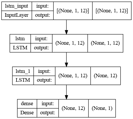
The network architecture includes:
- An input layer matching the window size
- Two hidden LSTM layers with 12 neurons each
- An output layer producing a scalar prediction
The number of neurons is chosen empirically, balancing training time and forecast accuracy. The output layer uses a single neuron with linear activation to predict the next time step's metric.
Generating Predictions
I trained the model on a two-year time series and predicted the next three months with weekly frequency. For comparison, I used a naive predictor that assumes the next value will match the current one (v(t+1) = v(t)). I calculated prediction errors (SMAPE) for the training set, test set, and naive predictor.
trainPredict = model.predict(train_X)
testPredict = model.predict(test_X)
naive = numpy.roll(test_y, 2)
# calculate root mean squared error
print(f"SMAPE for train: {round(smape(train_y, trainPredict[:, 0]),2)})")
print(f"SMAPE for test: {round(smape(test_y, testPredict[:, 0]),2)})")
print(f"SMAPE for naive: {round(smape(test_y, naive),2)})")
Results Analysis
The predictions are far from perfect. The actual market data is much more volatile than our model's forecasts. While the predictions attempt to follow the general trend of the actual data, they often contain significant errors.
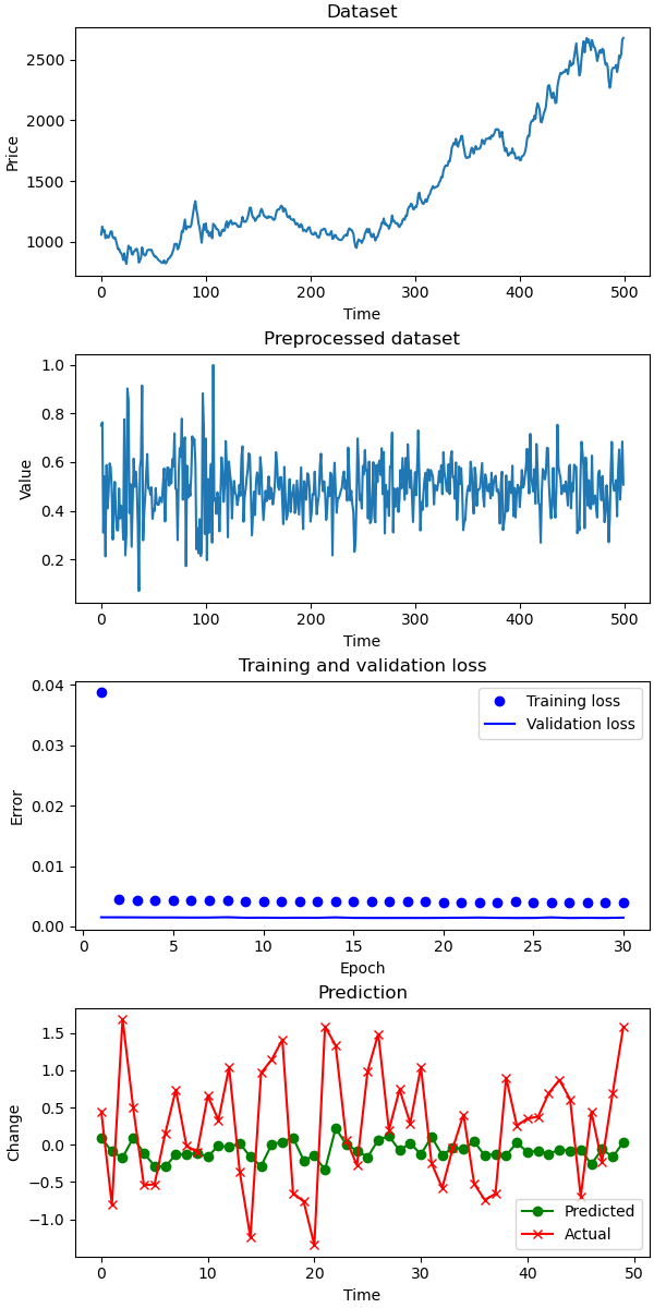
Comparing SMAPE (Symmetric Mean Absolute Percentage Error) values, the LSTM model still outperforms the naive predictor:
SMAPE for test:  6
SMAPE for naive: 8
Testing on Artificial Data
You might wonder if the model itself is flawed or if there's a bug in the code. To verify, we tested the LSTM on artificial data: a sinusoidal wave with a regular, predictable pattern.
def get_sin_wave():
    my_wave = np.sin(np.arange(0, 110, .1))
    return my_wave
SMAPE for test: 16
SMAPE for naive: 36

As expected, the model's prediction of the sinusoidal wave is nearly perfect. This suggests financial market data is far too complex and unpredictable for our simple LSTM network.
Key Takeaways
Our out-of-the-box LSTM model produces unsatisfactory results for stock price prediction. While it outperforms a naive predictor, it still makes significant errors—for example, predicting price increases when prices actually decrease, and vice versa.
LSTMs excel at time series prediction in fields like weather forecasting, electricity consumption prediction, and network traffic analysis. However, financial markets exhibit fundamentally different statistical properties than these natural phenomena. A common view is that in financial markets, past performance does not reliably predict future returns. Trading stocks has been compared to driving a car while looking only in the rear-view mirror—dangerous, given the unpredictable events ahead.
Investing can be seen as a form of information arbitrage, where success depends on having access to unique data or insights that other market participants lack. Trying to outperform the market using standard machine learning techniques and publicly available data is unlikely to succeed. Without a unique information advantage, you're more likely to waste time and resources with little or no return on investment.
This doesn't mean LSTMs can never predict stock prices. There are numerous ways to improve the model:
- Tune layer parameters
- Adjust the sliding window size (which also changes the input layer dimensions)
- Modify the architecture by adding more layers or incorporating other network types (like convolutional neural networks) to preprocess the data
The Complete Code
Input data — place in the same directory as the Python file.