ARMA process predicts the future taking into account past values and errors. When making predictions, we often reach the past to find a pattern which can repeat itself in the future. Such patterns may have roots in seasons, days (business days and weekends), or time of day (day and night). However, rarely does same pattern happen multiple times. Unexpected events related to politics, the economy and daily life in general, disrupt any ready-to-use templates. Therefore, we need models like ARMA that simultaneously use past data as a template for estimates and can also include unpredictable events distorting this template.
What is ARMA
The name ARMA is short for Autoregressive Moving Average. It comes from merging two simpler models – the Autoregressive, or AR, and the Moving Average, or MA. ARMA predicts the future taking into account a linear combination of past values and errors. The ARMA is only suitable for univariate time series without trend and seasonal components. If your data is more complex, but still has a linear dependency between past values, you have to pre-process the data before feeding the model or use more advanced process, e.g. ARIMA.
Prediction with the AR part
The AR (autoregressive) model explains a variable future value using its past or so called lagged values. The AR models the next step in the time series as a linear function of the observations at prior time steps.
The AR have a single parameter p which specify the number of lags in the model
The mathematical formulation of an AR(p) model is as follows:
where
- value to be predicted
- past values
- white noise
- weight of the past values
Prediction with the MA part
The Moving Average works comparably to the AR model: it uses past values to predict the current value of the variable. A moving average (MA) process of order q is a linear combination of the q most recent past white noise terms, which is defined by
where
- value to be predicted
- white noise
- weight of the white noise values
Joining AR and MA – prediction with ARMA
When used together, we call these concatenated blocks as the ARMA process. ARMA can use the past value and the prediction errors from the past ARMA stands for an Autoregressive Moving Average. As shown below, ARMA combines autoregression (AR) and moving average (MA) models into one block.
ARMA examples
As you can see, the ARMA can have different values for the lag of the AR and MA processes. For example
- ARMA(1, 0) model has an AR order of 1 (p= 1) and an MA order of 0 (q=0). This is just an AR(1) model
- The MA(1) model is the same as the ARMA(0, 1) model
- ARMA(3, 1) has an AR order of 3 lagged values and uses 1 lagged value for the MA.
Data acquisition
Firstly, we get the data. I selected a small-cap index from one of the Eastern European markets. Why not something more popular? Because the more popular data have fewer anomalies, making it harder to find inefficiencies.
My data is a time frame with several columns. I indexed, filtered and converted it to weekly frequency because of clearer autocorrelation at a higher scale. Finally, I computed the percentage change of the index to obtain a stationary time series. Finally, I divided the data into two sets: x_train and x_test, which are input parameters of the forecasting algorithms.
# File with price data
EQ = r'swig80.txt'
# Column's names
COL_DATE = ''
COL_OPEN = ''
COL_CLOSE = ''
COL_LOW = ''
COL_HIGH = ''
# Learning parameters
TEST_RATIO = 0.95
TRAIN_SIZE = 80
def get_data():
"""
Get all files in a given directory and its directories
"""
df = pd.read_csv(EQ)
# Convert data in string to date
df[COL_DATE] = df[COL_DATE].apply(pd.to_datetime, format="%Y%m%d")
# The whole data history is not necessary to predict next week
df = df[df[COL_DATE] >= '2017-01-01']
# Make a date an index of the frame
df.set_index(COL_DATE, inplace=True)
# Change the frequency from days to weeks
df = df.resample('1w').agg({COL_OPEN: 'first', COL_HIGH: 'max',
COL_LOW: 'min', COL_CLOSE: 'last'})
# Compute the percentage changes
df['change'] = df[COL_CLOSE].pct_change()*100
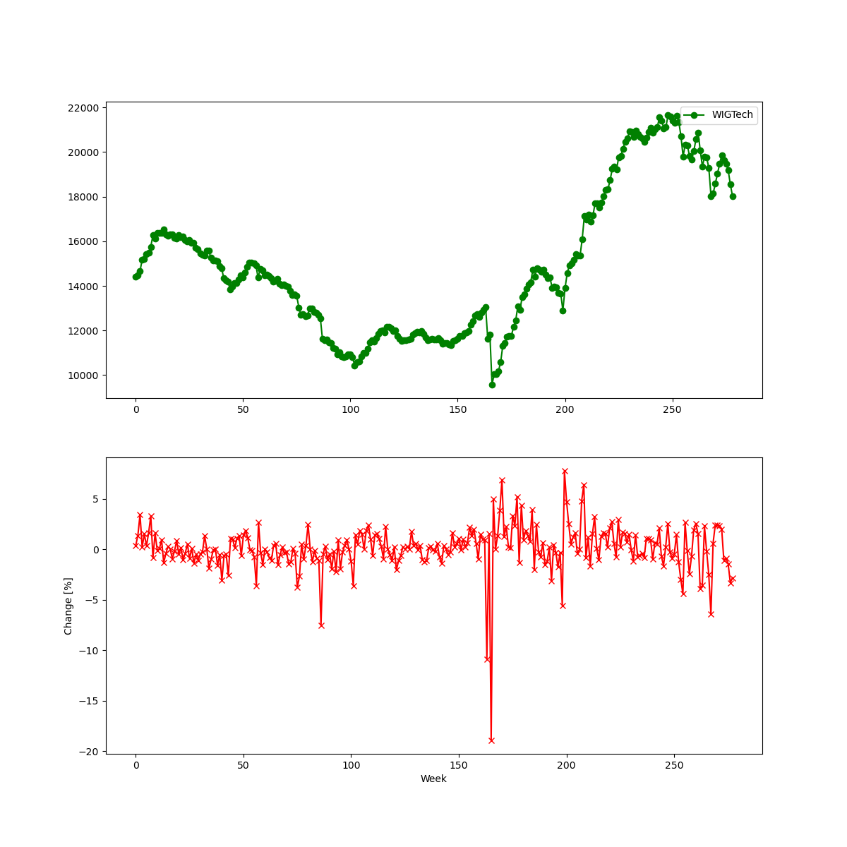
plot_eq(df[COL_CLOSE].to_numpy(), df['change'][1:].to_numpy())
return(df['change'][1:].to_numpy())
Finally, get_data() produces the time series which is an input to my prediction algorithms.
Predictions of prices with ARMA
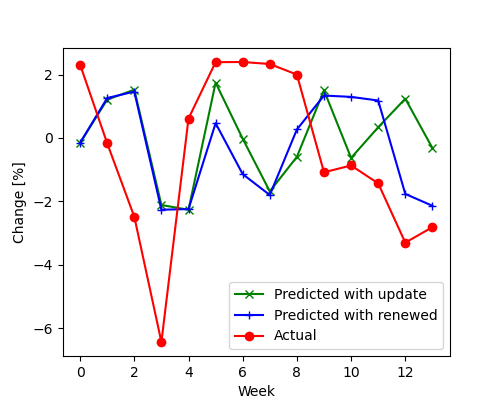
I supplied the model with the two-year length time series and predicted the next three months with a weekly frequency.
The first algorithm uses the update function. After every predicted value, this function “refreshes” the model parameters, uncovering the new observations. In the beginning, I created the auto_arima model. Then, in the loop, I predict the next values and refresh the model with the actual value new_ob taken from x_test set. From the differences between x_test and fc I computed prediction errors.
def forecast_with_update(x_train, x_test):
    auto_arima = pm.auto_arima(
            x_train, seasonal=False, stepwise=False,
            approximation=False, n_jobs=-1)
    print(auto_arima)
    forecasts = []
    for new_ob in x_test:
        fc, _ = auto_arima.predict(n_periods=1, return_conf_int=True)
        forecasts.append(fc)
        # Updates the existing model with a small number of MLE steps
        auto_arima.update(new_ob)
    print(f"Mean squared error: {mean_squared_error(x_test, forecasts)}")
    print(f"SMAPE: {pm.metrics.smape(x_test, forecasts)}")
    return forecasts
In the second approach, instead of updating, I recreated the model. Thus, in every loop, I replace the old model with a completely new one with updated data. This approach is much slower and updating the model. For more details about the differences between updating and creating a new model for every iteration, see the auto_arima documentation.
def forecast_with_new(x_train, x_test):
    forecasts = []
    print("Iterations {}".format(x_test.size))
    for new_ob in x_test:
        # Recompute the whole model
        auto_arima = pm.auto_arima(
                x_train, seasonal=False, stepwise=False,
                approximation=False, n_jobs=-1)
        fc, _ = auto_arima.predict(n_periods=1, return_conf_int=True)
        forecasts.append(fc)
        print("Iteration")
        x_train = np.append(x_train[1:], new_ob)

    print(f"Mean squared error: {mean_squared_error(x_test, forecasts)}")
    print(f"SMAPE: {pm.metrics.smape(x_test, forecasts)}")
    return(forecasts)
Results
In both cases, the prediction results are not satisfactory. The prediction does not follow the actual values. It seems that the data is more complicated and has non-linear dependencies, which the ARMA cannot model. Building a new model for every prediction did not help. To improve the results, one may consider to
- change the x_test size
- take different data, e.g. different indexes or equities
The whole code
Input data (put in the same directory as the Python file)