You probably read stories about artificial neural networks which predict stock prices. Some of them are even published as scientific papers. These algorithms were supposed to make their owners rich. Supposedly, it was enough to construct the network, feed it with stock prices, and get prices for the next hour, day or even a week. Is there any truth in such stories?

Over the past few years, numerous impressive accomplishments have been made through the application of deep learning techniques. Deep neural networks were successfully applied to tasks in which traditional machine learning algorithms could not succeed – large-scale image classification, autonomous driving, and superhuman performance when playing traditional games such as Go or classic video games. Almost yearly, we can observe the introduction of a new network type that has better prediction accuracy.
LSTM network
An LTSM is a recurrent artificial neural network (ANN) which can learn long-range dependencies in data. Compared to other types of ANNs, LSTM can learn and remember over long sequences. LSTM ANNs respond to the short-term memory problem of recurrent ANNs. Namely, a recurrent ANN has difficulties retaining data from earlier computations because it misses information about long-memory dependencies. An LSTM ANN handles this problem by allowing its memory cells to select when to forget certain information, thus achieving the optimal time lags for time series problems.
For this purpose, the LSTM uses a memory block which contains cells with self-connections, memorizing the temporary state and three adaptive, multiplicative gates: the input, the output, and the forget, to control information flow in the block. The gates can learn to open and close, enabling LSTM memory cells to store data over long periods, which is desirable in time series prediction with long temporal dependency. Multiple memory blocks form a hidden layer. An LSTM ANN consists of an input layer, at least one hidden layer and an output layer.
Data acquisition
The data are the same as in the previous post. As a result, we obtain a time series representing the percentage difference between the weekly prices of the equity.
Data preparation
Scale transformation
Similarly to other artificial neural networks, LSTM expects data to be within the scale of the activation function used by the network. The default activation function for an LSTM is the hyperbolic tangent, which outputs values between -1 and 1. Using scikit-learn transform classes, we transform our data set to the range [-1, 1] using the MinMaxScaler class.
dataset = dataset.reshape(-1, 1)
scaler = MinMaxScaler(feature_range=(-1, 1))
scaler.fit(dataset)
dataset = scaler.transform(dataset)
dataset = dataset.squeeze()
The MinMaxScaler class requires data in a matrix format with rows and columns, so we reshape our arrays before transforming. After the data scaler.transform() scales dateset into (-1, 1) range, we convert it to its original shape by removing the earlier added dimension. For this purpose, we use ndarray.squeeze().
Shape adjustment
The most common way to feed time series data into an ANN is to break the whole sequence into consecutive input windows and then get the ANN to predict the window or the single data point immediately following the input window. Thus, if we have an exemplary time series
we want to convert it to the format X, y, where X is a vector which holds the moving window and y is the value to be predicted. Table 1 shows the converted vector V with a window size 2.
| X | y | ||
|---|---|---|---|
| Row | V[t-1] | V[t] | V*[t+1] |
| 1 | 1 | 2 | 3 |
| 2 | 2 | 3 | 4 |
| 3 | 3 | 4 | 5 |
| … | … | … | … |
| 7 | 7 | 8 | 9 |
The code below transforms the time series into an array.
def to_windows(ts, window):
    x, y = [], []
    for i in range(len(ts)-window-1):
        a = ts[i:(i+window)]
        x.append(a)
        y.append(ts[i + window])

    return numpy.array(x), numpy.array(y)
The function takes:
- univariate time series ts, which is to be transformed into X, Y array and
- the window variable, which denotes the length of the X vector.
Within the loop, we slice our time series ts into len(ts)-window-1
vectors of length window and extract every vector v from the time series v = ts[i:(i+window)]. We append the vector v to the list x obtaining the left part of the array presented in Table 1. To the Y column, we assign the value ts[i + window] we want to predict. As an output of the function, we obtain numpy.array(x), numpy.array(y) which represents Table 1.
After acquiring data, we convert it to the array form
dataset = get_data("data/swig80.txt")
window = 6
X, y = to_windows(dataset, window)
The data returned by the to_windows look like this:
TrainX
trainX.round(1)

array([[ 0.4,  1.4,  3.4,  0.2,  1.5,  0.3],
       [ 1.4,  3.4,  0.2,  1.5,  0.3,  1.6],
       [ 3.4,  0.2,  1.5,  0.3,  1.6,  3.3],
       ...,
       [ 2.4,  5.2, -1.3,  4.4,  0.9,  1.9],
       [ 5.2, -1.3,  4.4,  0.9,  1.9,  1.4],
       [-1.3,  4.4,  0.9,  1.9,  1.4,  0.8]])
TrainY
array([  1.6,   3.3,  -0.8,   1.6,  -0.1,   0.1,   0.9,  -1.3,  -0.4,
...
5.2,  -1.3,   4.4,   0.9,   1.9,   1.4,   0.8,   3.9])
To feed our neural network, we must reformat it adding dimension
X = numpy.expand_dims(X, axis=1)
As the result, we obtain:
X
trainX.round(1)

array([[[ 0.4,  1.4,  3.4,  0.2,  1.5,  0.3],
       [ 1.4,  3.4,  0.2,  1.5,  0.3,  1.6],
       [ 3.4,  0.2,  1.5,  0.3,  1.6,  3.3],
       ...,
       [ 2.4,  5.2, -1.3,  4.4,  0.9,  1.9],
       [ 5.2, -1.3,  4.4,  0.9,  1.9,  1.4],
       [-1.3,  4.4,  0.9,  1.9,  1.4,  0.8]]])
y
array([[  1.6,   3.3,  -0.8,   1.6,  -0.1,   0.1,   0.9,  -1.3,  -0.4,
...
5.2,  -1.3,   4.4,   0.9,   1.9,   1.4,   0.8,   3.9]])
You can also achieve the same results using timeseries_dataset_from_array. However, the function hides the building mechanism of the sliding window.
Division into training, validation and test
To avoid model over- or under-learning from training data, we need to check how good is the learning process and how well the model generalizes. For this purpose we divided the input data into training, validation, and testing subsets.
train_X, test_X, train_y, test_y = train_test_split(
    X, y, test_size=0.10, shuffle=False)
train_X, validate_X, train_y, validate_y = train_test_split(
    train_X, train_y, test_size=0.20, shuffle=False)

Dataset division
Training
After our data is ready, we can build the LSTM.
def build_model(train_X, train_y, validate_X, validate_y, window):
    """
    Build the predictive model
    Parameters
        train_X: training independent vectors
        train_y: training dependent variables
        validate_X, validate_y: validation independent and dependent vectors
        window: sliding window lenght
    :return
        model - predictive model
        history - training history
    """
    model = Sequential()
    model.add(LSTM(12, recurrent_dropout=0.5, return_sequences=True, input_shape=(1, window)))
    model.add(LSTM(12, recurrent_dropout=0.5, input_shape=(1, window)))
    model.add(Dense(1))
    model.compile(loss='mean_squared_error', optimizer='adam')
    history = model.fit(
            train_X, train_y, epochs=30, verbose=2,
            validation_data=(validate_X, validate_y))
    return(model, history)
The network architecture consists of an input layer whose size is set to window size, two hidden layers with 12 neurons each, and an output layer which produces a scalar value. The number of neurons is usually chosen mostly empirically. There is a trade-off between optimal training time and forecast accuracy involved in the selection of this parameter. The network requires a single neuron in the output layer with a linear activation to predict the given metric at the next time step.
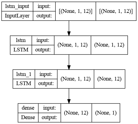
LSTM architecture
Predictions
I supplied the model with the two-year length time series and predicted the next three months with a weekly frequency. For the comparison, I used a naive predictor, which predicts the next value to be the same as the current one: v(t+1) = v(t). Then, I computed errors for train, test sets and the naive predictor.
trainPredict = model.predict(train_X)
testPredict = model.predict(test_X)
naive = numpy.roll(test_y, 2)
# calculate root mean squared error
print(f"SMAPE for train: {round(smape(train_y, trainPredict[:, 0]),2)})")
print(f"SMAPE for test: {round(smape(test_y, testPredict[:, 0]),2)})")
print(f"SMAPE for naive: {round(smape(test_y, naive),2)})")
Results
The prediction is far from perfect. The actual data is more volatile than the predicted. Although, the prediction tries to follow the actual data, in many cases it make significant errors.
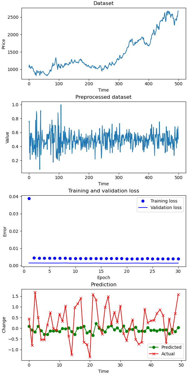
Prediction for a stock index
Comparing the prediction errors SMAPE, the LSTM is still better than the naive predictor v(t+1) = v(t).
SMAPE for test:  6
SMAPE for naive: 8
Predicting artificial data
You may think: Probably the ANN is faulty or Maybe there something wrong with the code?. So, let’s test the code on artificial data. The data is a sinusoidal wave — a regular pattern which should be easier to approximate by our ANN.
def get_sin_wave():
    my_wave = np.sin(np.arange(0, 110, .1))
    return my_wave
SMAPE for test: 16
SMAPE for naive: 36
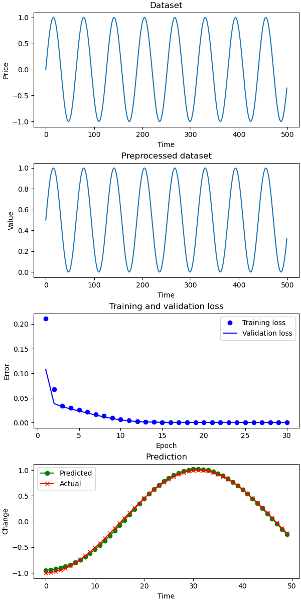
Prediction for a sine wave
As you see, the prediction is nearly perfect. It seems that the market data are far too complex for our network.
Summary
The out-of-the-box model does not have satisfactory results. Although it is better than a naive predictor, it makes many prediction mistakes, e.g. it predicts an increase in price while the actual price decreases or vice versa.
The prediction is successfully applied to many fields such as weather, electricity consumption, network traffic etc. However, financial markets have different statistical characteristics than these natural phenomena. One of the popular views is, that in the case of markets, past performance is not a good predictor of future returns. Trading the markets can be compared to driving a car – there are too many unpredictable events ahead and looking in the rear-view mirror is a bad way to drive.
Investing can be considered a form of information arbitrage, which means gaining an advantage by having access to certain data or insights that other market participants don’t have. However, trying to use common machine learning techniques and publicly available data to outperform the markets is not a good idea. This is because you won’t have any unique information advantage over others, and you are likely to waste your resources and time with little or no return on investment.
It does not mean that it in certain circumstances predicts stock prices. You can try to tune the network in many different ways
- Change its layers parameters, see here the possibilities
- Manipulate with the sliding window size which changes also the size of the input layer
- Change its architecture, add more layers related, or add a layer from another type of network like convolution ANNs to additionally process the data
So, you can experiment and please let me know in the comment section if you find something interesting.
The whole code
Input data — put in the same directory as the Python file.