Features:
- Calculates capital gains and estimates tax using FIFO and LIFO
- Long and short positions: stocks, ETFs, crypto-currencies,
- Detailed and configurable reports - you can filter the report by date or by product/equity name
- Export the reports to a spreadsheet for further custom analysis
- Supports CSV files or copy-pasted transaction data
- Flexible import formats - specify the file format and save it as a template
- Free, no subscription, no data harvesting, no advertising.
How it works?
Upload your data
Upload a file with your transaction data or simply copy-paste it.
Don’t worry about transaction format.
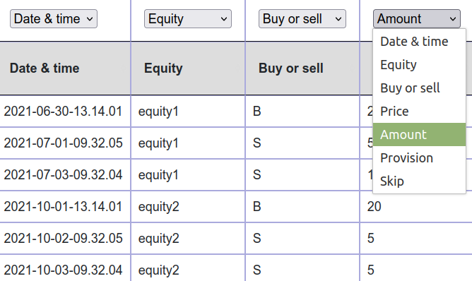
Describe the format
Interactively describe the format of your data.
Provide information using a simple interactive form.
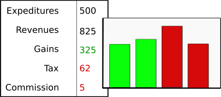
Analyze results
- Check out your capital gains, taxes, and commissions.
- Calculate the statistics for the whole portfolio and individual equities. Investigate every equity and every transaction in your portfolio